Introduction to Financial Risk Management (FRM)
The FRM application is integrated with Temenos Transact and is delivered as a pre-packaged and upgradeable risk management software. It enables the clients to:
- Measure and monitor financial risks
- Reduce cost of capital and compliance
- Improve profitability in lending
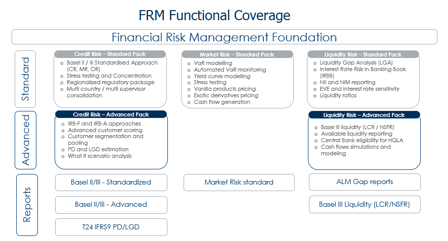
The FRM application consists of three modules and they are:
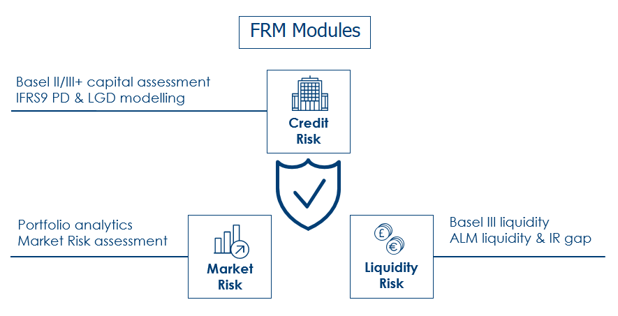
The modules are segregated to various features. The below capture illustrates:
- Features of FRM modules
- Functional areas supported by each feature
- Various approaches or methodologies for risk management
Market Risk Overview
The Market Risk module is an advanced market risk analytical tool that supports banks to measure and monitor market risk across banks trading and bank book .
The module has a pre-configured interface with Temenos Transact and is designed to operate in both batch and interactive mode.
The below screen capture illustrates the process flow and list of various features available in the module.
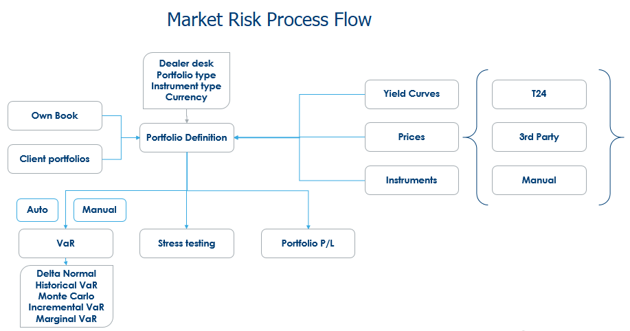
The features included in this module are:
- Yield Curve Modelling
- Delta Normal VaR
- Calculation of VaR using Historical Simulation
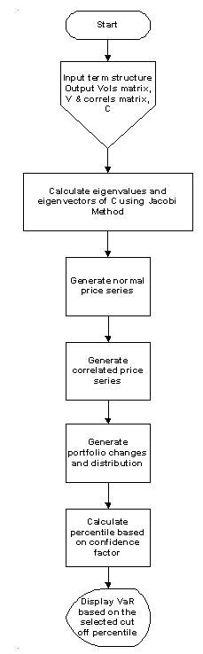
- Calculation of VaR using Monte Carlo Simulation
- Incremental and Marginal VaR
- Derivation of Volatilities and Correlations
- VaR Back Testing
- Cash Instruments Stress Testing
- Pricing of Illiquid Debt Instruments
- Fixed Rate Bond
- Floating Rate Bonds
- Derivative Pricing
- FX Forwards
- Swaps
- Options
In addition, this section describes the various calculation models that are used in the Market Risk module.
Calculation Models
The below table provides the list of calculation models.
| Parameter | Methodology |
|---|---|
|
Yield curve interpolation |
Linear interpolation |
|
Volatility |
Standard deviation of price history Standard deviation of daily price change Standard deviation of log of daily price change |
|
Risk factor mapping for cash instruments |
Weighted duration based |
|
Statistical distribution type |
Normal distribution |
|
Risk factor generation method |
Cash Non cash |
|
Stress testing |
Parallel shifts in: Par rate Zero rate Discount rate |
|
Yield curve models |
Par (input rate) Discount rate (bootstrapped) ZCYC Forward rate |
|
Monte Carlo VaR |
Generating eigenvalues, eigenvectors using Jacobi method (single factor) |
|
Bond pricing |
Fixed rate Floating rate (discount margin) |
|
Derivative pricing |
FX FWD SWAP (CRS, IRS) Options (American, European, Bermudian - Black Scholes and Binomial tree) |
|
Value at Risk |
Parametric Historical simulation Monte Carlo Marginal and incremental |
Yield Curve Modelling
This section describes the yield curve models.
Discount Rates calculated using the bootstrapping methodology (Forward Substitution). The first step is to calculate discount factors for all short-term points (MM term points generally < 1 year). Then follows the forward substitution methodology to bootstrap all the discount factors for each term point.

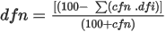
Where,
cfn = is the coupon of the n-year bond
dfi = is the discount factor for that time period
dfn = is the discount factor for the entire period, from which we derive the zero-rate.
Forward Rates
Once all the discount rates are calculated, forward rates are calculated from the zero rates derived from the discount rate calculated above.
Where,
ZCn = Zero Rate for n period
The system uses linear interpolation methodology for interpolating yields between term points. The closed ended formula for linear interpolation used is:
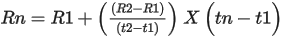
Where,
Rn = Interpolated yield
R1 = Previous term point Yield
R2 = Next term point yield
T1 = Previous term point days
T2 = Next term point days
Tn = interpolated yield term point days
Value at Risk
Value at Risk is the maximum amount that can be lost on a portfolio over a period of time at a given level of confidence. This section describes about value at risk models.
In the system, parametric VaR is calculated for portfolio using the following matrix algebra:
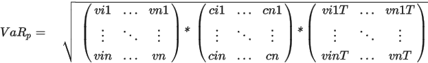
Where,
VaRP = Portfolio VaR
V = Vector matrix of position VaR
C = Correlation Matrix of the assets in the portfolio
VT = Transpose of the Vector matrix
Historical simulation takes the portfolio of assets at a particular point in time and then revalues the portfolio using the historical prices of the assets in the portfolio. The portfolio revaluation produces a distribution of P&L which is then used to determine the portfolio VaR at a given confidence factor. This process can get computationally intensive if there is large number of assets in the portfolio and price history over a significant time period.
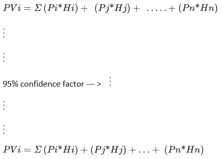
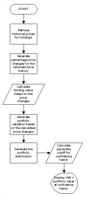
Where,
Pn = Price of asset i
Hn = Holding of asset i
Monte Carlo simulation involves artificially generating large set of events (correlated price changes) from which VaR is derived. This involves two steps: Generate random numbers and then converting them into set of normally distributed price changes. And for multi asset portfolio this is done using the Jacobi’s method of generating EignValues and EignVectors for the correlation matrix.
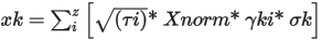
Where,
Xk = correlated random price change for asset k with a normal distribution and the volatility of the asset k
 = square root of the eigenvalue for the asset k
Xnorm = random price change from a normally distributed series
 = the kth element of the eigenvector for the ith asset
 Volatility of the kth asset
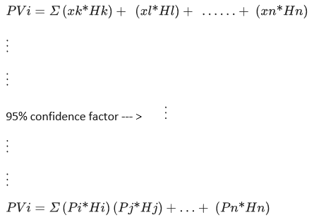
Where,
Xk = Price of asset calculated
Hn = Holding of asset
Debt Instruments Pricing
This section describes the various debt instruments pricing calculation models.
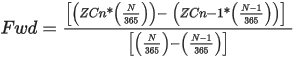
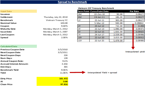
For pricing illiquid debt securities over a benchmark issue, system uses the interpolated yield of the benchmark issue for the maturity date of the security. Then using the closed ended formula, price is calculated based on the interpolated yield and the spread.
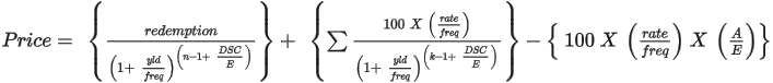
Where,
Redemption = redemption value
Yield = Interpolated Benchmark Yield + spread
Frequency = frequency of coupon payment
DSC = number of days from settlement to next coupon date
E = number of days in coupon period in which the settlement date falls
N = number of coupons payable between settlement date and redemption date
A = number of days from beginning of coupon period to settlement date
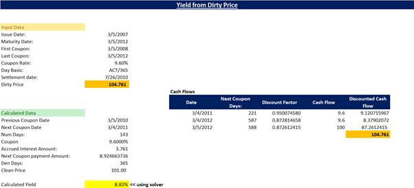
Yield is calculated from the pricing function using an iterative process by keeping the yield variable to match the user defined dirty / clean price with the price computed with yield. The yield is changed until the estimated price given the yield is close to price.
Bond prices tend to revert to par as it nears the maturity date. To price a floating rate bond, discount margin is used. An investor can make the additional yield if the bond is priced at a discount and vice a versa, if the security is priced at a premium, then the DM will equal reference rate less the DM.
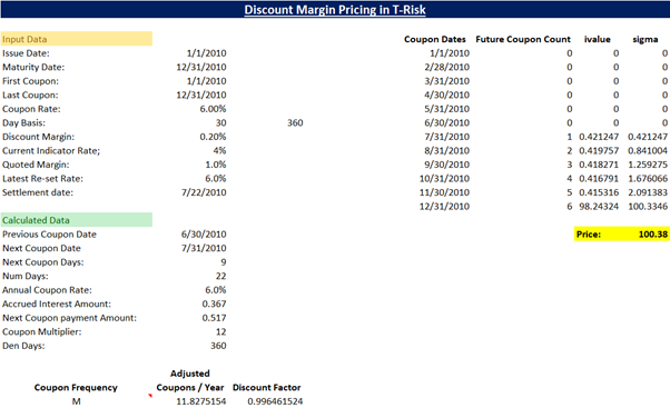


Where,
DM = Discount Margin
Df = Discount Rate
IR = Current Indicator Rate
QM = Quoted Margin
n = Period till maturity
Cash flow allocation:
Cash flow allocation in the system is completed using the Weighted Duration methodology. The below flowchart gives the complete flow of the calculation process.
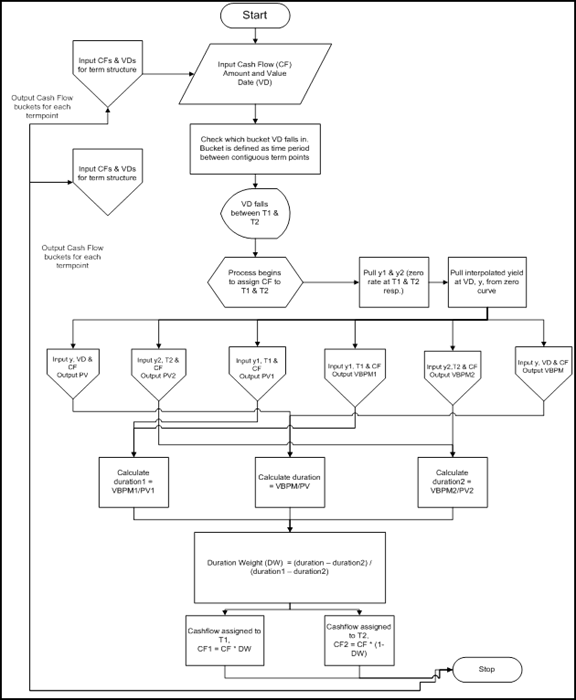
Below are the procedure for calculating the price of a fixed rate bond:
- Calendar date wise cash flows have to be arrived.
- Present Value Factor has to be determined based on YTM and Frequency.
- Calculate the present value of future cash flows.
- Sum them up to get full value of a bond, also called Dirty Price.
Calculate interest accrued and subtract its value from Dirty Price to get Clean Price of a bond.
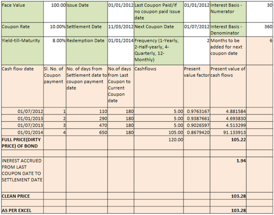
System Illustration:
Following are the procedure to calculate price for a fixed rate bond via Market Risk module screens.
Select Home > Master Data Configuration > Portfolio Configuration > Instruments to access the Instruments screen.
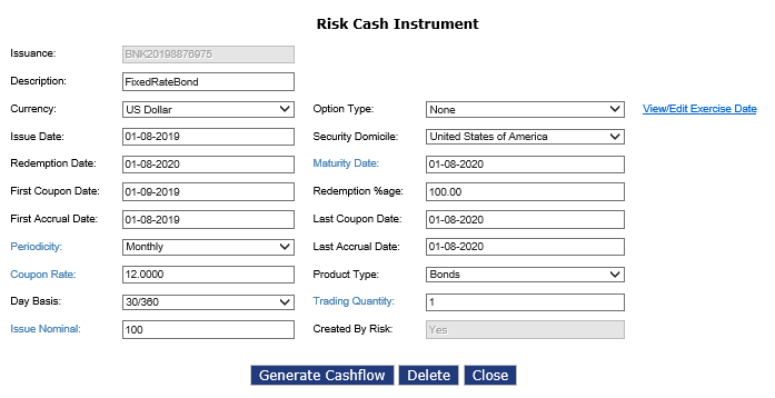
Enter or select required values in the respective fields. Click Generate Cashflow.
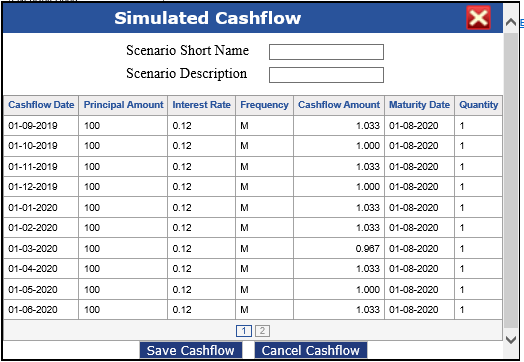
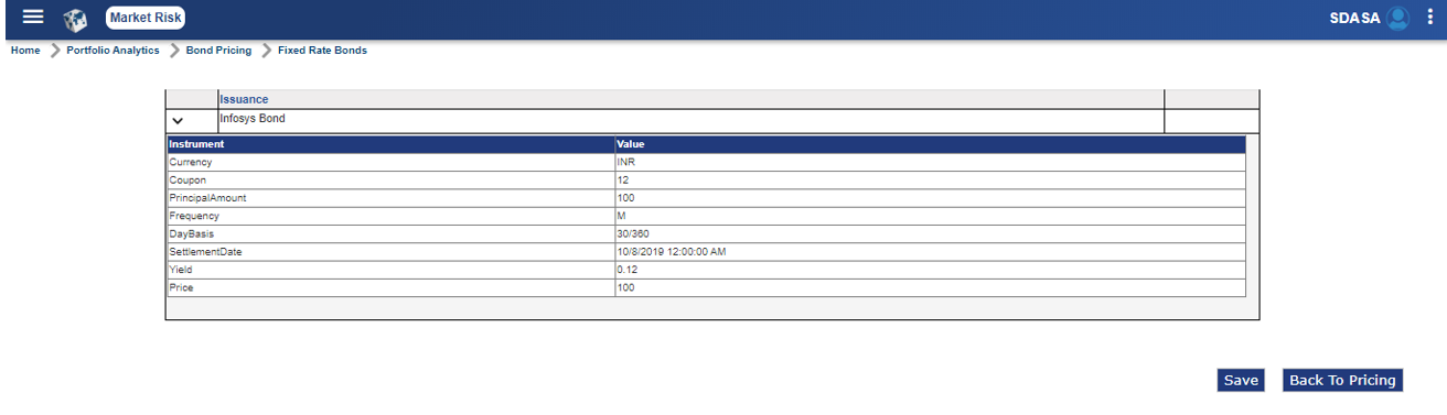
Bond Pricing:
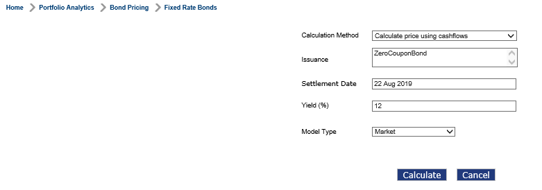
Select Home > Portfolio Analytics > Bond Pricing > Fixed Rate Bonds to access the Fixed Rate Bonds screen.
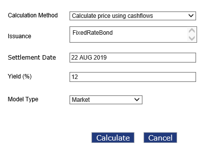
Enter or select values in the fields given below:
| Field | Description |
|---|---|
| Calculation Method | Select ‘Calculate price using cash flows’ option from the drop-down. |
| Issuance | Select an issuance by selecting the check box corresponding to that issuance. User can select one or more issuance to price them in single process. |
| Settlement Date | Enter the settlement date. The date has to be on or after current system date along with Yield or the discounting factor to discount cash flows. Denote the date on which the investor of the bond/instrument obtains possession of the instrument after buying. |
| Yield (%) | Enter a percentage based on the expected rate of return on a bond in line with the changing market conditions. |
| Model Type | Select a model type. The available options are ‘Market’ and ‘Scenario’. Market is related to the cash flows that have been generated when instrument was created with initial parameters and scenario denotes the scenario related cash flows. |
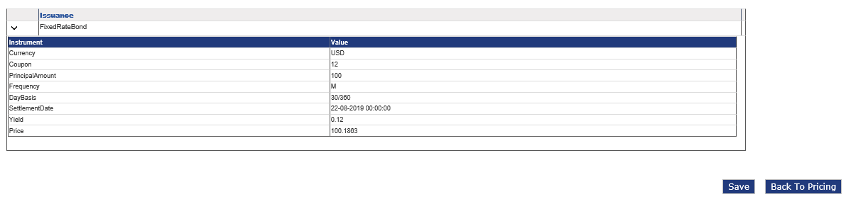
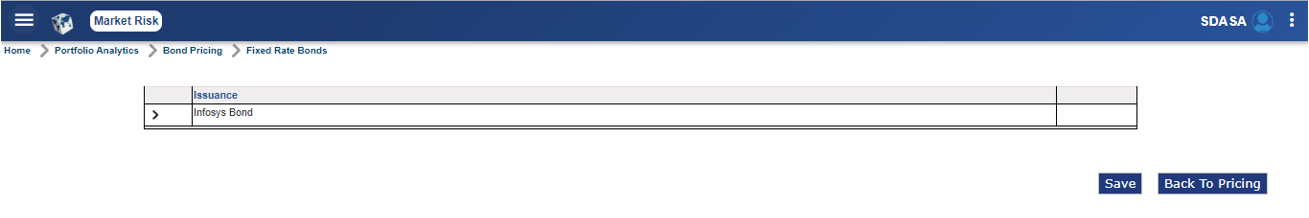
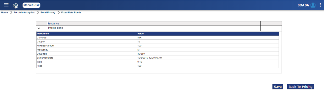
After entering the fixed rate bond details, click Calculate Price. The Fixed Rate Bond screen is displayed with the price details. The user can expand the Issuance field to view the price details.
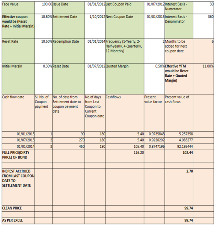
Below are the procedure for calculating the price of a floating rate bond:
- Calendar date wise cash flows have to be arrived. For Floating Rate Bonds, cash flows is based on Reset Rate and Initial Margin put together, which can be called as “Effective Coupon Rate”.
- Present Value Factor is based on YTM and Frequency of payments. This is arrived at by adding Reset Rate and Quoted Margin.
- Calculate the present value of future cash flows.
- Sum them up to get full value of a bond, also called Dirty Price.
- Calculate interest accrued and subtract its value from Dirty Price to get Clean Price of a bond.
System Illustration:
Following are the procedure to calculate price for a floating rate bond via Market Risk module screens.
Select Home > Portfolio Analytics > Bond Pricing > Floating Rate Bonds to access the Floating Rate Bonds screen.
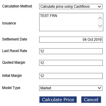
Enter or select values in the fields given below:
| Field | Description |
|---|---|
| Calculation Method | Select ‘Calculate price using cash flows’ option from the drop-down. |
| Issuance | Select an issuance by selecting the check box corresponding to that issuance. User can select one or more issuance to price them in single process. |
| Settlement Date | Enter the settlement date. The date has to be on or after current system date along with Yield or the discounting factor to discount cash flows. Denote the date on which the investor of the bond/instrument obtains possession of the instrument after buying. |
| Last Reset Date | Enter the date on which interest rate on a floating rate bond is decided and this field is not applicable for fixed rate bond. |
| Quoted Margin | Enter additional percentage above reset rate to be summed up along with reset rate for Yield To Maturity. |
| Initial Margin | Enter additional percentage above the reference rate/reset rate. |
| Model Type | Select a model type. The available options are ‘Market’ and ‘Scenario’. Market is related to the cash flows that have been generated when instrument was created with initial parameters and scenario denotes the scenario related cash flows. |
After entering the floating rate bond details, click Calculate Price. The Floating Rate Bond screen is displayed with the price details. The user can expand the Issuance field to view the price details.
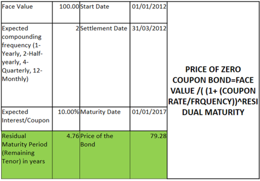
Below are the procedure for calculating the price of a Treasury Bill:
- Arrive at the residual maturity of the bond in actual days.
- Discount the face value by (1 + YTM adjusted for the no. of days).
- The assumption is that year consists of 360 days as it is the normal convention.
System Illustrations:
Following are the procedure to calculate price for a Treasury bill via Market Risk module screens.
Select Home > Master Data Configuration > Instruments to access the Instruments screen.
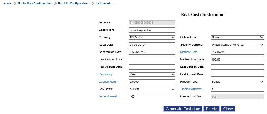
Enter or select required values in the respective fields. Click Generate Cashflow.
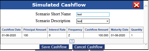
Select Home > Portfolio Analytics > Bond Pricing > Fixed Rate Bonds to access the Fixed Rate Bonds screen.
Enter or select values in the fields given below:
| Field | Description |
|---|---|
| Calculation Method | Select ‘Calculate price using cash flows’ option from the drop-down. |
| Issuance | Select an issuance by selecting the check box corresponding to that issuance. User can select one or more issuance to price them in single process. |
| Settlement Date | Enter the settlement date. The date has to be on or after current system date along with Yield or the discounting factor to discount cash flows. Denote the date on which the investor of the bond/instrument obtains possession of the instrument after buying. |
| Yield (%) | Enter a percentage based on the expected rate of return on a bond in line with the changing market conditions. |
| Model Type | Select a model type. The available options are ‘Market’ and ‘Scenario’. Market is related to the cash flows that have been generated when instrument was created with initial parameters and scenario denotes the scenario related cash flows. |
After entering the fixed rate bond details, click Calculate Price. The Fixed Rate Bond screen is displayed with the price details. The user can expand the Issuance field to view the price details.
Derivative Pricing
This section describes the various derivative pricing calculation models.
An FX forward contract is an agreement to purchase or sell a set amount of a foreign currency at a specified price for settlement at a predetermined time in the future.
System uses following model to value an FX Forward:
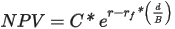
Where,
NPV - FX trade mark-to-market in valuation currency,
C - Cash flow in foreign currency,
d - Number of days from calculation date to settlement date,
r - Continuous zero coupon rate on settlement date in domestic currency,
rf - Continuous zero coupon rate on settlement date in foreign currency.
B - Interest basis (360 or 365)
Below table is an example describing the FX forward calculation:
| Parameter | Working |
|---|---|
| Deal Date | 16-Jun-18 |
| Deal Rate / Strike Rate (K) | 1.3 |
| Spot Date | 28-Jun-18 |
| Spot Rate (S) | 1.35 |
| Maturity Date (M) | 27-Feb-19 |
| CCY bought | USD |
| Amount bought | 1,350,000.00 |
| Yield for bought CCY | 0.50% |
| CCY sold | EUR |
| Amount sold | -1,000,000.00 |
| Yield for sold CCY | 2% |
| Revaluation Rate ( R ) | 1.3349 = 1.35 * EXP ^ (0.5% - 2%) * (9 / 12) |
An interest rate swap (IRS) is an agreement between two counterparties to exchange fixed for floating cash flows. Although the notional principal is not exchanged in a swap, the assumption is, without changing the value of the swap that the two counterparties pay each other the same notional amount. Another possibility is, a portfolio consisting of one fixed leg, which is equivalent to a fixed-coupon bond, and one floating leg, which is equivalent to an FRN.
IRS is calculated on the below model:

Where,
- fi is the estimated forward rate on the ith period of the floating side
- ri is the continuously compounded zero coupon rate of the ith receiver cash flow
- BR is the receiver interest basis (360 or 365)
- Mi is the number of days in period i (using the appropriate day count convention) of the floating side
- di is the time to maturity from the As Of Date to the ith cash flow date of the floating side
- NR is the receiver notional amount
- Ml is the number of periods on the floating side
- k is the payer’s fixed rate
- rj is the continuously compounded zero coupon rate of the jth payer cash flow
- BP is the payer interest basis (360 or 365)
- Mj is the number of days in period j (using the appropriate day count convention) of the fixed side
- dj is the time to maturity from the As Of Date to the jth cash flow date of the fixed side
- Mx is the number of periods on the fixed side
- NP is the payer notional amount
Currency swaps are swaps that consists element of IR risk as well as FX risk. The valuation model is same as IRS. Refer below tables for valuation examples:
| Parameter | Value |
|---|---|
| USD | 1,000,000.00 |
| INR | 50,000,000.00 |
| Coupon-USD | 2% |
| Coupon-INR | 6% |
| Long position (Leg 1) | USD |
| Short position (Leg 2) | INR |
| Frequency | 2 |
| Maturity Date | 20-Aug-18 |
| As on date | 14-Jun-15 |
| Index-USD | Libor-USD |
| Index-INR | YC1 |
| Spot Rate(USD/INR) | 65.00 |
| Valuation of Leg1 | |||||
|---|---|---|---|---|---|
|
Cash Flow Dates |
Cash Flows |
Residual Maturity |
Yield (Interpolated) |
DF |
PV |
| 20-Aug-18 | 1,000,000.00 | 3.1836 | 4.0455 | 0.8792 | 879,159.04 |
| 20-Aug-18 | 100.00 | 3.1863 | 4.0469 | 0.8790 | 87.90 |
| 20-Feb-18 | 10,000.00 | 2.6904 | 3.6776 | 0.9058 | 9,057.96 |
| 20-Aug-17 | 10,000.00 | 2.1863 | 3.3469 | 0.9294 | 9,294.40 |
| 20-Feb-17 | 10,000.00 | 1.6904 | 3.1014 | 0.9489 | 9,489.24 |
| 20-Aug-16 | 10,000.00 | 1.1863 | 2.9096 | 0.9661 | 9,660.72 |
| 20-Feb-16 | 10,000.00 | 0.6877 | 2.8188 | 0.9808 | 9,808.03 |
| 20-Aug-15 | 10,000.00 | 0.1836 | 2.8000 | 0.9949 | 9,948.73 |
| Sum | 936,506.03 | ||||
| Valuation of Leg2 | |||||
|---|---|---|---|---|---|
|
Cash Flow Dates |
Cash Flows |
Residual Maturity |
Yield (Interpolated) |
DF |
PV |
| 20-Aug-18 | 50,000,000.00 | 3.1836 | 8.2810 | 0.7683 | 38,412,841.96 |
| 20-Aug-18 | 15,000.00 | 3.1863 | 8.2812 | 0.7681 | 11,521.18 |
| 20-Feb-18 | 1,500,000.00 | 2.6904 | 8.2452 | 0.8011 | 1,201,576.52 |
| 20-Aug-17 | 1,500,000.00 | 2.1863 | 8.1986 | 0.8359 | 1,253,849.41 |
| 20-Feb-17 | 1,500,000.00 | 1.6904 | 8.1428 | 0.8714 | 1,307,108.56 |
| 20-Aug-16 | 1,500,000.00 | 1.1863 | 8.0949 | 0.9084 | 1,362,655.20 |
| 20-Feb-16 | 1,500,000.00 | 0.6877 | 8.0925 | 0.9459 | 1,418,805.56 |
| 20-Aug-15 | 1,500,000.00 | 0.1836 | 8.1000 | 0.9852 | 1,477,862.25 |
| Sum | 46,446,220.62 | ||||
INR equivalent PV of Leg 1 = 936,506.03 * 65 = 60,872,89.00
PV of Leg 2 = 47,588,257.09
Value of Swap (L-S) = 13,284,634.91
Options valuation using Black-Scholes model
Options valuation using Black-Scholes model would use the standard formula:


Where,


Below tables are working examples:
| Parameter | Value |
|---|---|
| Spot Price (S) | 40 |
| Risk free rate of interest (r) | 5% |
| Strike price (K) | 45 |
| Maturity Date/Expiry Date | 8-Feb-17 |
| Valuation Date | 8-Feb-16 |
| Volatility(σ) | 20% |
| Rate of Interest (Rf) | 3% |
| Residual Maturity (t) | 1.002739726 |
| Reporting Currency | INR |
| CCY1 | USD |
| CCY2 | INR |
| Parameter | Value |
|---|---|
| d1 | -0.078 |
| d2 | -0.278 |
| Call Price | 1.491 |
| Put Price | 5.476 |
The binomial tree valuation model is performed by means of a binomial lattice (tree), for a number of time steps between the valuation and expiration dates. Each node in the lattice represents a possible price of the underlying at a given point in time.
Working example for a 1-step binomial tree
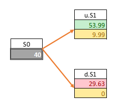
Below table is a working example for 1-step binomial tree:
| Parameters | |
|---|---|
| Stock Price (S0) | 40 |
| Exercise Price (X) | 44 |
| Interest Rate (r) | 4% |
| Volatility (σ) | 30% |
| Time to Maturity (t) | 1 |
| Number of Steps | 1 |
| Dividend Yield | 0 |
| Calculations | |
|---|---|
| Time Interval (t) | 1 |
| Up movement (u) | 1.349859 |
| Down movement (d) | 0.740818 |
| Up probability (p) | 0.492566 |
| Down probability (q) | 0.507434 |
| Discount Factor | 0.740818 |
| Price of a Call (C) | 4.729847 |
Where,

The same principle is used for modelling for puts and multi-step binomial tree model.
Pricing of MBS and ABS Using Discounted Cash Flows
This section describes the types of Mortgaged Backed Securities (MBS) and pricing of MBS. Read Configuring MBS Bonds for more information.
Generate Cash Flows for Bond with Option - Callable and Puttable
Callable Bond - A callable bond (also called redeemable bond) is a type of bond (debt security) that allows the issuer of the bond to retain the privilege of redeeming the bond at some point before the bond reaches its date of maturity. Hence the issuer has option to buy back on the stated exercise dates at the stated strike price, issuer will exercise the option when the yield is maximum among the various exercise dates.
Puttable Bond - Puttable bond (put bond, putable or retractable bond) is a bond with an embedded put option. The holder of the puttable bond has the right, but not the obligation, to demand early repayment of the principal. The put option is exercisable on one or more specified dates. A bond that is issued with option to the buyer of the bond to sell back to issuer on the stated exercise dates at the stated strike price, buyer will exercise the option when the yield is minimum among the various exercise dates.
Read Pricing Bond with Option for more information.
In this topic